PyTorch Practical for Linear Neural Network
PyTorch Practical for Linear Neural Network
- Implementing Linear Regression with PyTorch
- Implementing Softmax Regression with PyTorch
1. Implementing Linear Regression with PyTorch
1.1. 目标
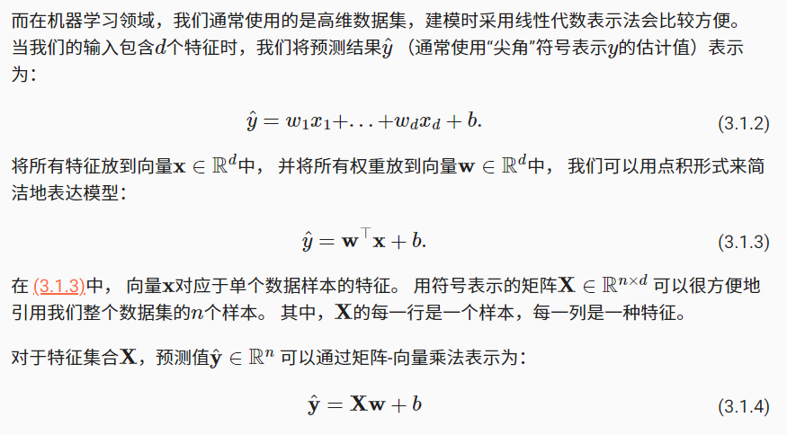
整体目标:预测
实例:根据房屋的面积和房龄来估算房屋价格

给定一个数据集,我们的目标是寻找模型的权重w和偏置b,使得根据模型做出的预测大体符合数据里的真实价格。
1.2. 合成数据集
import torch

def synthetic_data(w, b, num_examples):
    """生成y=Xw+b+噪声"""
    """num_examples:样本数量
        w:权重向量
        b:偏置
    """
    X = torch.normal(0, 1, (num_examples, len(w))) # torch.Size([1000, 2])
    y = torch.matmul(X, w) + b # torch.Size([1000])
    y += torch.normal(0, 0.01, y.shape) # torch.Size([1000])  加上噪声
    return X, y.reshape((-1,1)) # torch.Size([1000, 2]), torch.Size([1000, 1])
- torch.normal(means,std,out=None)
- 参数:
- means(Tensor):均值
- std(Tensor):标准差
- out(Tensor):可选的输出张量,指定Tensor的size是几行几列
- 返回:
- 返回一个张量,从给定均值、标准差的离散正太分布中抽取随机数
- 此处解读:
- 均值为0,标准差为1,输出张量num_examples行,len(w)列
- 参数:
true_w = torch.tensor([2, -3.4])
true_b = 4.2
features, labels = synthetic_data(true_w, true_b, 1000) # torch.Size([1000, 2]), torch.Size([1000, 1])
1.3. 数据加载
from torch.utils import data

def load_array(data_arrays, batch_size, is_train=True):
    dataset = data.TensorDataset(*data_arrays)
    return data.DataLoader(dataset, batch_size, shuffle=is_train)
batch_size = 10
data_iter = load_array((features, labels), batch_size)
每一批次的数据有10条,示例如下:
[tensor([[-0.5176,  0.6470],
         [ 0.7657, -0.0239],
         [ 1.2130, -0.2022],
         [ 0.7047,  1.4854],
         [-0.3069,  2.0228],
         [ 1.3954,  1.4201],
         [ 0.2607, -0.0518],
         [ 1.3602, -0.3472],
         [ 0.2915,  0.4973],
         [ 1.0556,  0.8510]]),
 tensor([[ 0.9683],
         [ 5.8210],
         [ 7.3061],
         [ 0.5730],
         [-3.2839],
         [ 2.1581],
         [ 4.9031],
         [ 8.1074],
         [ 3.0919],
         [ 3.4130]])]
1.4. 定义网络
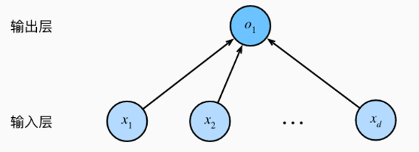 线性回归是一个单层神经网络。对于线性回归,每个输入都与每个输出相连,我们将这种变换称为全连接层(full-connected layer)或称为稠密层(dense layer)。
输入为x1,...,xd,因此输入层中的输入数(或称为特征维度,feature dimensionality)为d。
输出为O1,因此输出层中的输出数是1。
from torch import nn

net = nn.Sequential(nn.Linear(2,1))

# 初始化参数:通过_结尾的方法将参数替换,从而初始化参数
# 我们指定每个权重参数应该从均值为0、标准差为0.01的正态分布中随机采样,偏置参数将初始化为零
net[0].weight.data.normal_(0, 0.01) # 通过net[0]选择网络中的第一个图层
net[0].bias.data.fill_(0)

print(net)
网络结构为:
Sequential(
  (0): Linear(in_features=2, out_features=1, bias=True)
)
- Sequential类将多个层串联在一起。当给定输入数据时,Sequential实例将数据传入到第一层,然后将第一层的输出作为第二层的输入,以此类推。
- torch.nn.Linear(in_features,out_features,bias=True) 用于设置网络中的全连接层
- in_features:每个输入样本的大小
- out_features:每个输出样本的大小
- bias:偏置,默认有偏置
- 从输入输出的张量的shape角度来理解,相当于一个输入为[batch_size, in_features]的张量变换成了[batch_size, out_features]的输出张量
1.5. 定义损失函数
loss = nn.MSELoss()
1.6. 定义优化器
trainer = torch.optim.SGD(net.parameters(), lr=0.03)
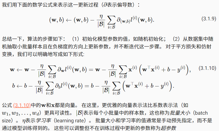
梯度下降(gradient descent):通过不断地在损失函数递减的方向上更新参数来降低误差,几乎可以优化所有深度学习模型。
小批量随机梯度下降:原本计算损失函数(数据集中所有样本的损失均值)关于模型参数的导数(梯度)会很慢,因为每次更新参数要遍历整个数据集。因此,我们通常随机抽取一小批样本就更新一次参数,这一小批是由固定数量的训练样本组成的。
小批量随机梯度下降算法是一种优化神经网络的标准工具,PyTorch在optim模块中实现了该算法的许多变种。
当我们实例化一个SGD实例时,我们要指定优化的参数(可通过net.parameters()从我们的模型中获得)以及优化算法所需的超参数字典。
小批量随机梯度下降只需要设置学习率lr值,指在梯度下降的方向上走多大步伐,这里设置为0.03。
1.7. 模型训练
num_epochs = 3
for epoch in range(num_epochs): # 每一轮 (在每个迭代周期里,我们将完整遍历一次数据集)
    for X,y in data_iter: # 每一批次(获取一个小批量的输入和相应的标签)
        # 此处X,y分别是features和labels的一个小批量
        l = loss(net(X), y) # 通过调用net(X)前向传播,生成预测,并计算损失
        trainer.zero_grad() # 初始化梯度为0
        l.backward() # 通过进行反向传播来计算梯度
        trainer.step() # 通过调用优化器来更新模型参数
    # 为了更好的衡量训练效果,我们计算每个迭代周期后的损失,并打印它来监控训练过程
    l = loss(net(features), labels) # 一轮完成后,算整体数据的损失
    print(f'epoch{epoch+1},loss{l:f}')
输出结果为:
epoch1,loss0.000239
epoch2,loss0.000103
epoch3,loss0.000103
1.8. 评估效果
w = net[0].weight.data
b = net[0].bias.data
print('估计的w:', w.reshape(true_w.shape))
print('w的估计误差:', true_w - w.reshape(true_w.shape))
print('估计的b:', b)
print('b的估计误差:',true_b - b)
输出结果为:
估计的w: tensor([ 2.0000, -3.3994])
w的估计误差: tensor([ 2.1219e-05, -5.6791e-04])
估计的b: tensor([4.2010])
b的估计误差: tensor([-0.0010])
2. Implementing Softmax Regression with PyTorch
2.1. 目标
整体目标:分类
实例:图像分类,给定图像,识别是哪一个类别

与线性回归一样,softmax回归也是一个单层神经网络。softmax回归的输出层也是全连接层。
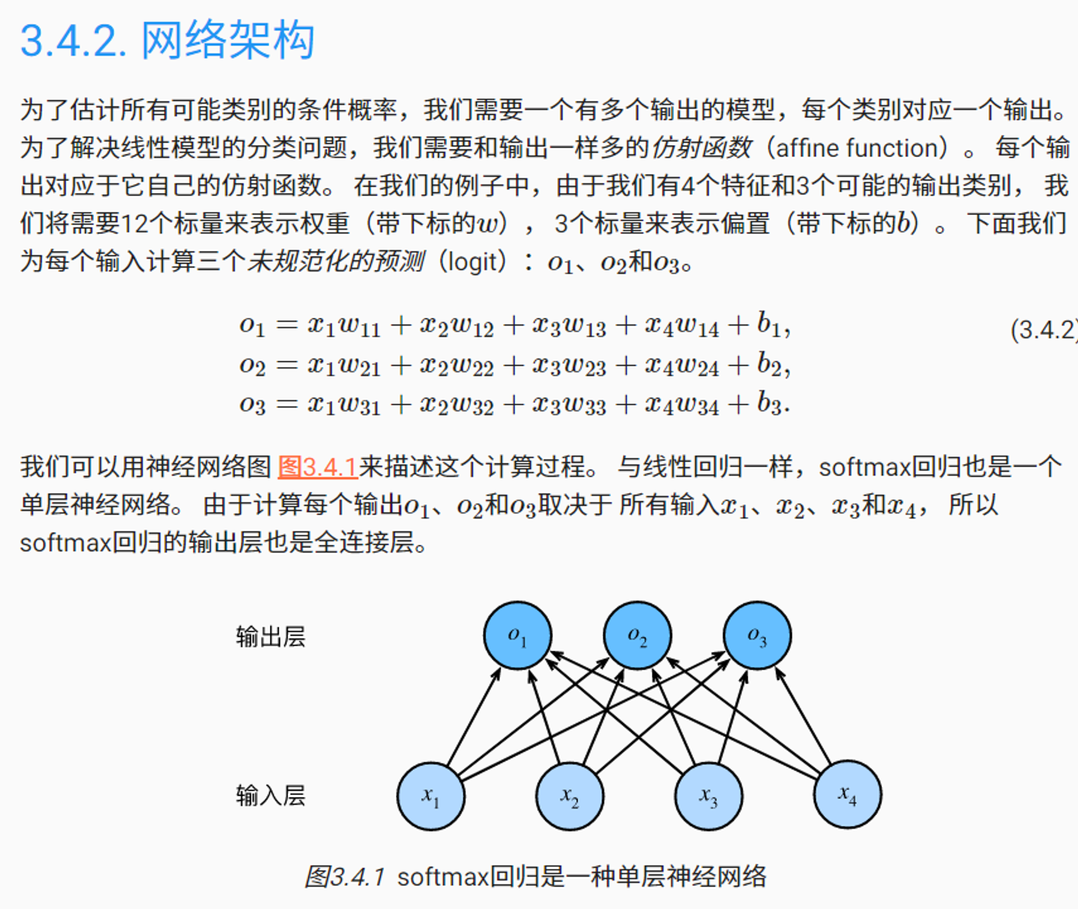
softmax函数:softmax函数能够将未规范化的预测变换为非负数并且总和为1,可以视为求概率分布。 softmax运算不会改变未规范化的预测o之间的大小次序,只会确定分配给每个类别的概率。
2.2. 数据集介绍
Fashion-MNIST由10个类别的图像组成, 每个类别由训练数据集(train dataset)中的6000张图像 和测试数据集(test dataset)中的1000张图像组成。 因此,训练集和测试集分别包含60000和10000张图像。 测试数据集不会用于训练,只用于评估模型性能。
Fashion-MNIST中包含的10个类别,分别为t-shirt(T恤)、trouser(裤子)、pullover(套衫)、dress(连衣裙)、coat(外套)、sandal(凉鞋)、shirt(衬衫)、sneaker(运动鞋)、bag(包)和ankle boot(短靴)。
每个输入图像的高度和宽度均为28像素。 数据集由灰度图像组成,其通道数为1。
2.3. 数据加载
import torchvision
from torch.utils import data
from torchvision import transforms

def load_data_fashion_mnist(batch_size, resize=None):
    """下载Fashion-MNIST数据集,然后将其加载到内存中"""
    trans = [transforms.ToTensor()]
    if resize:
        trans.insert(0, transforms.Resize(resize))
    trans = transforms.Compose(trans)
    mnist_train = torchvision.datasets.FashionMNIST(
        root="../data", train=True, transform=trans, download=True)
    mnist_test = torchvision.datasets.FashionMNIST(
        root="../data", train=False, transform=trans, download=True)
    return (data.DataLoader(mnist_train, batch_size, shuffle=True,
                            num_workers=4),
            data.DataLoader(mnist_test, batch_size, shuffle=False,
                            num_workers=4)) # 使用4个进程来读取数据
batch_size = 256
train_iter, test_iter = load_data_fashion_mnist(batch_size)
for X, y in train_iter:
    print(X.shape, X.dtype, y.shape, y.dtype) # 每个图片形状为torch.Size([1, 28, 28]),对应一个0-9的标签
    break
输出为:
torch.Size([256, 1, 28, 28]) torch.float32 torch.Size([256]) torch.int64
2.4. 定义网络并初始化参数
from torch import nn
# 在线性层前定义了展平层(flatten),来调整网络输入的形状
# 输入层为28*28=784个神经元,输出层为10种类别的神经元
# softmax回归的输出层是一个全连接层
net = nn.Sequential(nn.Flatten(), nn.Linear(784, 10))
# 初始化模型参数
def init_weights(m):
    if type(m) == nn.Linear:
        nn.init.normal_(m.weight, std=0.01) # 以均值0和标准差0.01随机初始化权重

net.apply(init_weights);
2.5. 定义损失函数
loss = nn.CrossEntropyLoss(reduction='none')
2.6. 定义优化器
import torch
trainer = torch.optim.SGD(net.parameters(), lr=0.1) # 使用学习率为0.1的小批量随机梯度下降作为优化算法
2.7. 模型训练
from matplotlib import pyplot as plt
from IPython import display
from matplotlib_inline import backend_inline

def use_svg_display():
    """使用svg格式在Jupyter中显示绘图"""
    backend_inline.set_matplotlib_formats('svg')

def set_axes(axes, xlabel, ylabel, xlim, ylim, xscale, yscale, legend):
    """设置matplotlib的轴"""
    axes.set_xlabel(xlabel)
    axes.set_ylabel(ylabel)
    axes.set_xscale(xscale)
    axes.set_yscale(yscale)
    axes.set_xlim(xlim)
    axes.set_ylim(ylim)
    if legend:
        axes.legend(legend)
        axes.grid()

class Animator:
    """在动画中绘制数据"""
    def __init__(self, xlabel=None, ylabel=None, legend=None, xlim=None,
                 ylim=None, xscale='linear', yscale='linear',
                 fmts=('-', 'm--', 'g-.', 'r:'), nrows=1, ncols=1,
                 figsize=(3.5, 2.5)):
        # 增量地绘制多条线
        if legend is None:
            legend = []
        use_svg_display()
        self.fig, self.axes = plt.subplots(nrows, ncols, figsize=figsize)
        if nrows * ncols == 1:
            self.axes = [self.axes, ]
        # 使用lambda函数捕获参数
        self.config_axes = lambda: set_axes(
            self.axes[0], xlabel, ylabel, xlim, ylim, xscale, yscale, legend)
        self.X, self.Y, self.fmts = None, None, fmts

    def add(self, x, y):
        # 向图表中添加多个数据点
        if not hasattr(y, "__len__"):
            y = [y]
        n = len(y)
        if not hasattr(x, "__len__"):
            x = [x] * n
        if not self.X:
            self.X = [[] for _ in range(n)]
        if not self.Y:
            self.Y = [[] for _ in range(n)]
        for i, (a, b) in enumerate(zip(x, y)):
            if a is not None and b is not None:
                self.X[i].append(a)
                self.Y[i].append(b)
        self.axes[0].cla()
        for x, y, fmt in zip(self.X, self.Y, self.fmts):
            self.axes[0].plot(x, y, fmt)
        self.config_axes()
        display.display(self.fig)
        display.clear_output(wait=True)
class Accumulator:
"""在n个变量上累加"""
def __init__(self, n):
self.data = [0.0] * n
def add(self, *args):
self.data = [a + float(b) for a, b in zip(self.data, args)]
def reset(self):
self.data = [0.0] * len(self.data)
def __getitem__(self, idx):
return self.data[idx]
def accuracy(y_hat, y):
"""计算预测正确的数量"""
if len(y_hat.shape) > 1 and y_hat.shape[1] > 1:
y_hat = y_hat.argmax(axis=1)
cmp = y_hat.type(y.dtype) == y
return float(cmp.type(y.dtype).sum())
def evaluate_accuracy(net, data_iter):
"""计算在指定数据集上模型的精度"""
if isinstance(net, torch.nn.Module):
net.eval() # 将模型设置为评估模式
metric = Accumulator(2) # 正确预测数、预测总数
with torch.no_grad():
for X, y in data_iter:
metric.add(accuracy(net(X), y), y.numel())
return metric[0] / metric[1]
def train_epoch_ch3(net, train_iter, loss, updater):
"""训练模型一个迭代周期"""
# 将模型设置为训练模式
if isinstance(net, torch.nn.Module):
net.train()
# 训练损失总和、训练准确度总和、样本数
metric = Accumulator(3)
for X, y in train_iter:
# 计算梯度并更新参数
y_hat = net(X)
l = loss(y_hat, y)
updater.zero_grad()
l.mean().backward()
updater.step()
metric.add(float(l.sum()), accuracy(y_hat, y), y.numel())
# 返回训练损失和训练精度
return metric[0] / metric[2], metric[1] / metric[2]
def train_ch3(net, train_iter, test_iter, loss, num_epochs, updater):
"""训练模型"""
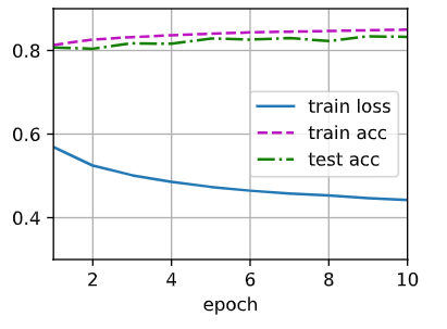
animator = Animator(xlabel='epoch', xlim=[1, num_epochs], ylim=[0.3, 0.9],
legend=['train loss', 'train acc', 'test acc'])
for epoch in range(num_epochs):
train_metrics = train_epoch_ch3(net, train_iter, loss, updater)
test_acc = evaluate_accuracy(net, test_iter)
animator.add(epoch + 1, train_metrics + (test_acc,))
train_loss, train_acc = train_metrics
assert train_loss < 0.5, train_loss
assert train_acc <= 1 and train_acc > 0.7, train_acc
assert test_acc <= 1 and test_acc > 0.7, test_acc
num_epochs = 10
train_ch3(net, train_iter, test_iter, loss, num_epochs, trainer)